
Executive Summary
Non-Governmental Organizations are not politically independent and usually suck up to major political parties to recieve funding and continue their operations. This project attempts to provide an alternative to boosting the funding status of NGOs by targeting individuals instead of bigger organizations. With growing middle class population, the contribution to NGO funds by common individuals has grown rapidly over the years. This is implemented by desiging a classification model using AWS SageMaker to predict the income status of an individual and thereby allowing the NGO to optimize their donation requests to individuals.
Project Overview
The NGO sector is now the eighth largest economy in the world worth over $1 trillion a year globally. It employees nearly 19 million paid workers, not to mention the countless volunteers. Despite its dominance, NGOs are not politically independent and the socio-economic and political factors play a really important role in its functioning. Another factor to note is that individual contribution to NGO funds has been on a steep rise over the past few years. The objective in this project is to identify if an individual earns more than 50k dollars or higher income bracket and request optimum donation amounts based on their incomes. This analysis can provide an efficient way for NGOs to have a substantial amount of donation by just targeting fewer but ‘right’ individuals.
Data Preparation
In order to achieve the objective, we perform a classic case of a classification
task. The dataset of individual information and their income level is fetched from the following UCI machine learning repository:
Individual Income Dataset - UCI Archives
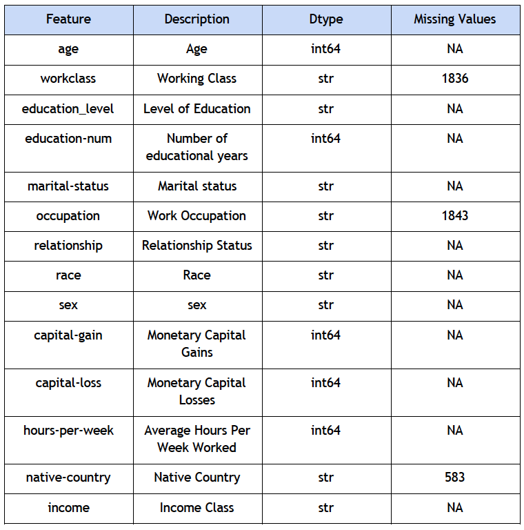
A. Description
B. Exploratory analysis
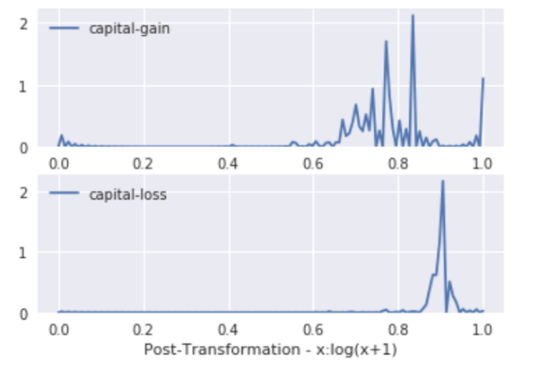
For the features capital gain and capital loss, we notice a fluctuating curve with random spikes at certain positions. Some capital gain data values are way beyond the mean value forming extreme outliers.

To prevent this from impeding the classification modeling process, we take a log transformation on these features. The issue here is that multiple data points have zero values in these features, and logarithm of 0 is undefined. Hence, we increment the value slightly and then obtain the log transformation as shown below to restrict the values between (0,1).
C. Dealing with missing values
Upon viewing our data, we found that we have multiple missing values in a few features represented by the string ‘?’. The count of these missing values is shown in the table above. We notice that most of the features are multi-valued categorical features and around 5 features are numeric. Overall, these variables can be intuitively interpreted to cause an effect in an individual’s income level. First glance at the dataset helps us conclude that certain features require transformations and cleaning. Initially, we hoped to find a statistical or machine learning based approach to impute these missing values. For example, using the mean of the column or using a classifier to impute values will allow us to keep these entries instead of deleting them.
However, using the mean of a column with categorical values is not possible. While using a classifier was still possible for these variables, the three columns that include missing values are workclass, occupation and native country. These variables are related to a person’s demographics, and would not make much sense to predict. The fact that we only have around 40,000 rows of data makes it unlikely that a classification would produce accurate results for these columns. For these reasons, we decided to cut our losses in terms of losing data points and removed all missing values from our dataset.
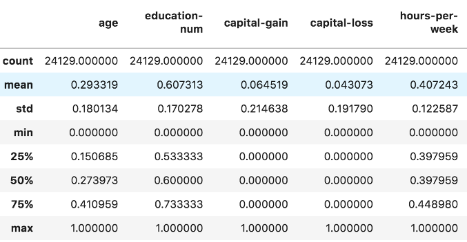
D. Scaling features
Algorithms like random forest and gradient tree boosting work best if the numeric values are standardized to prevent scaling issues when training the model. This is done by subtracting the mean and dividing by the standard deviation. The multi-valued categorical features are therefore one-hot encoded for the same principle.
E. Train-test split
To follow the guidelines for machine learning model building, we split out data in a training and test set. We used a split of 80/20, with 80% of the data going to training and 20% going to the test set. In order for consistency among our models, it was important to use the same data splits as well as using standardized variables for all three models.
Methodology
A. Architecture
AWS Sagemaker turned out to be our ideal choice since its offerings provided for a collectively exhaustive range for all our implementations. We used AWS S3 storage solution to load our dataset and created a notebook instance using the conda environment to run python and fetch the data from S3. We used the Linear model and XGBoost in-built training images offered by SageMaker to train the classification model and store the results in artifacts. We also developed a random forest implementation using the sklearn functionality and a separate script to feed it as an entry point into SageMaker. The models were deployed and the test data was used to make predictions and compare different models.
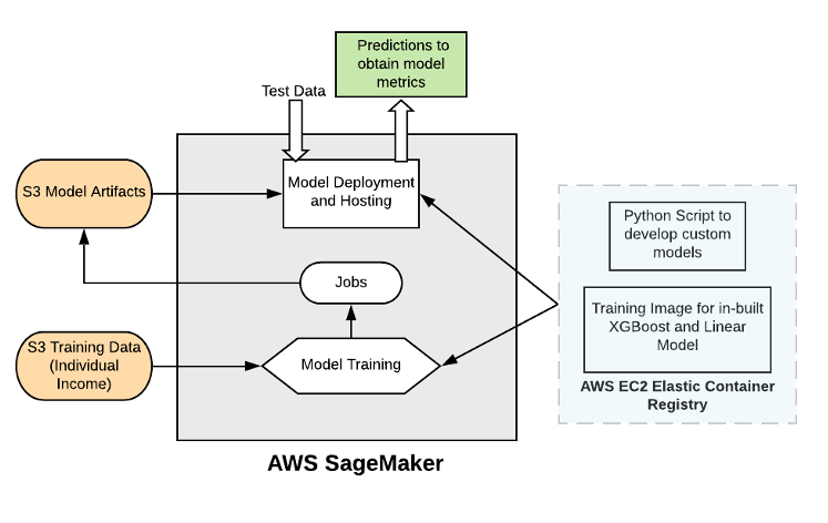 Implementation Architecture
B. Linear Model
While AWS/Sagemaker does not have a dedicated logistic regression model, it is possible to create a logit model using the linear-learner function. What differentiates the logistic regression in the function call is the “predictor_type” argument. Setting this to “binary_classifier” will cause the linear learner to predict for labels. The advantage of the linear learner model is that its prediction output can be set as both the probability and predicted label. This option was not available for both Random Forest and XGBoost, and our workaround will be discussed further in the report.
The steps to create a linear learner are identical to other AWS Sagemaker, however, the amount of possible hyperparameters is quite limited for this model. One important hyperparameter that separates linear learners from other models is the “L1” regularization parameter. Using this hyperparameter, we could penalize our model for excessive complexity and deal with overfitting. This was especially helpful since we were using a large amount of features after one-hot encoding. Another hyperparameter we used was “learning rate”, which controls how aggressively our function attempts to minimize our loss function. Since the optimization process of a linear model involves the use of gradient descent, the learning rate controls the size of the “steps” that the linear model takes when computing the iterative gradient of the loss function. A higher learning rate can cause the gradient descent to possibly miss the global minimum of the loss function, or converge to a local minimum before possibly finding the global minimum (which is the goal). Finally, we adjusted positive sample weights (increasing weight of samples with income >50k) and whether or not our model used bias.
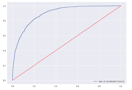
Even with adjusting these hyperparameters, this model was the worst performing out of the three we chose, based on all three metrics. This could be due to a multitude of factors, the most likely of these being that the other models were able to pick up non-linear relationships among some of the predictor variables which vastly improved their performance. Shown below is the Receiver Operator Curve(ROC):
 ROC-AUC Curve for linear model
C. Random Forest Model
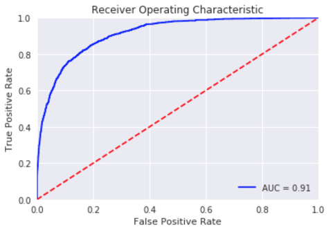
Since random forest is not offered as a training image directly by AWS SageMaker, we create a custom script using the Sklearn package and setting static hyperparameters to run the model. This is fed as an entry point to the sklearn model function in the SageMaker training instance to create a training job. This is then saved as an artifact. We extract the saved models to obtain the probability predictions on the test data to obtain various metrics like auc, precision and recall. The AUC shows a high bend in the curve exposing daylight between the blue and the trivial red curve, thus suggesting that this is a good model. We also obtain the top feature importances to identify the top attributes in the model performance.
 ROC-AUC Curve for random forest model
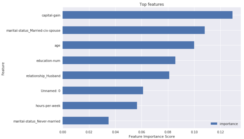
We notice that capital gain, marital status being a spouse and age are the top three features. The importance is distributed with a constant decrease in the top 10 features. We then tune the hyperparameters to improve the model performance. We use a larger set of trees to train the model and with higher minimum nodes in the leaf positions. We get a slightly different feature importance. Capital gains still is on the top followed by marital status, but age drops to a lower position and is overtaken by features like education years and if the individual is a husband.
D. XGBoost Model
Given the out-of-the-box managed model hosting and deployment in AWS SageMaker, XGBoost was an ideal choice for our implementation. Using the same set of features as used above, we initiate a training job on SageMaker on the pre-defined XGBoost training image. We also perform cross validation to find the best hyper-parameters.
Our best model is provides these parameters: eta= 0.2, gamma = 3, max_depth=5 and min_child_weight=6.
Step size shrinkage is used in updates to prevent overfitting. After each boosting step, we can directly get the weights of new features. The eta parameter actually shrinks the feature weights to make the boosting process more conservative.
Gamma is the minimum loss reduction required to make a further partition on a leaf node of the tree. The larger the value is, the more conservative the algorithm is.
Min_child_weight is the minimum sum of instance weight (hessian) needed in a child. If the tree partition step results in a leaf node with the sum of instance weight less than min_child_weight, the building process gives up further partitioning.
Max_depth is the maximum depth of a tree. Increasing this value will make the model more complex and more likely to overfit. 0 is only accepted in lossguided growing policy when tree_method is set as ‘hist’ and it indicates no limit on depth.
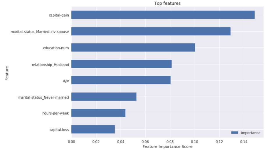
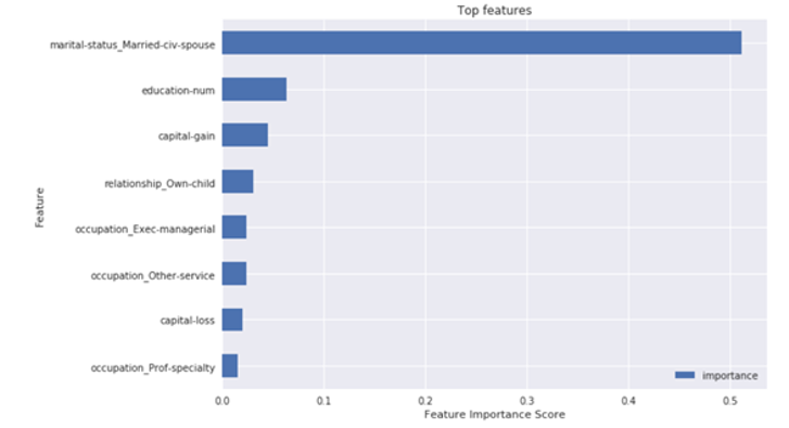
On plotting the feature importance, we see that the marital-status has highest importance. Followed by education and capital gain. Although the top features from XGBoost are similar to that of Random Forest, we see a substantial difference in feature importance of top 2 features in XGB. This is because the XGB runs on Boosting where it identifies the most important variable and focuses its learning improvement on this feature. Whereas, in RF the distribution is equally distributed as it uses bagging/bootstrap sampling for its learning process and this causes more distributed feature importance.
D. Model Comparison
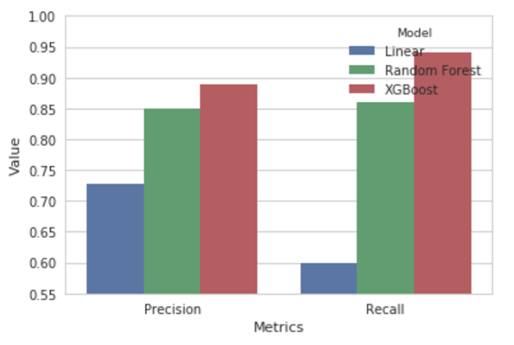
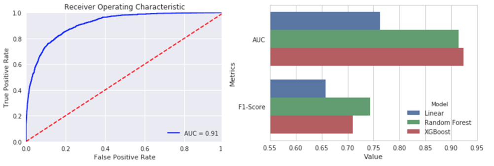
After obtaining all the three model predictions, we now compare different models based on various performance metrics. A side-by-side comparison of all the models based on precision and recall is shown alongside. Precision is basically defined as out of total positive predictions, how many are correct. Recall is the ratio of the correct predictions to the total actual positives. Our focus is having a high recall since we want to decrease the false negative predictions. Essentially, we do not want to lose out on an individual who has a high net worth and willing to donate more. Therefore it is fair to say that XGboost is the winner. We also compare our models on the basis of AUC on the test data. We see that it is pretty high compared to the trivial mean model. On the right side is side by side comparison of AUC and F1. Even though F1 is a little high for random forest, our main metric to decide the best model was AUC, and hence we chose XGBoost to make the final predictions of probabilities on the data.
Insights
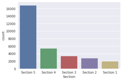
Once we obtain the best model predictions and the probabilities, We divide these probabilities into 5 bins named section 5-1. Section 1 having the highest probabilities and individuals with the highest income. The chart below is the distribution of individuals per section throughout the data.
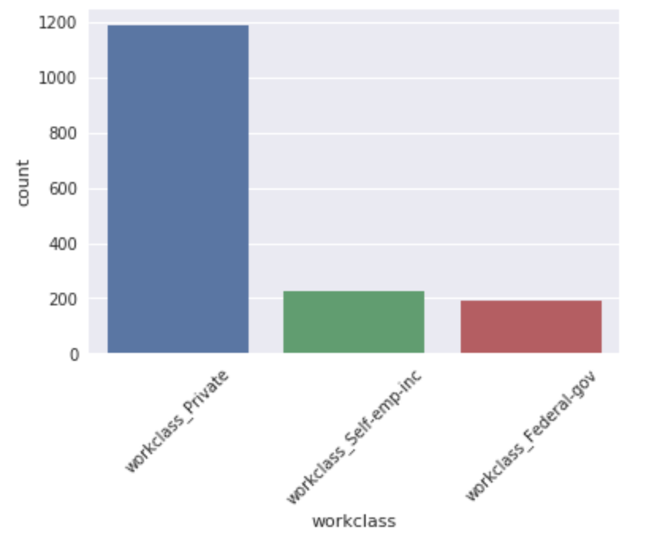
We also generate various summary inferences filtering out only section 1 individuals to target them specifically. This is done to identify the main attributes that result in high income. On the right side, you see the top working class of individuals in section 1. Most of them work in the private sector. Some individuals are also self employed and work for the federal government.
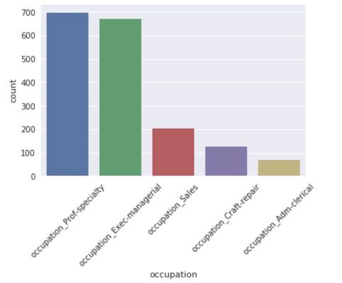
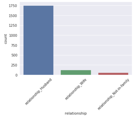
Occupations like professors or executive managerial positions were extremely high in section 1 compared to other occupations like sales, clerics etc. We also noticed that most of the individuals in section 1 were married husbands as shown in the right chart. As an NGO, we could use all these attributes and insights to target individuals and request appropriate donation amounts.
Click PDF to view more details on this project.
Ashish Gupta
Data Scientist | Engineer | Business Analyst
AI | ML | Analytics | Other Crazy Interests